
- 65
- 254 256
Marc Deisenroth
Registrace 13. 10. 2011
Video


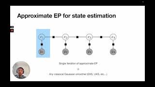
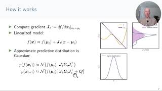
Iterative State Estimation in Non-linear Dynamical Systems Using Approximate Expectation Propagation
zhlédnutí 494Před 2 lety
video summarizing TMLR paper available at openreview.net/forum?id=xyt4wfdo4J

Jackie Kay: Fairness for Unobserved Characteristics
zhlédnutí 318Před 3 lety
Recent advances in algorithmic fairness have largely omitted sexual orientation and gender identity. We explore the concerns of the queer community in privacy, censorship, language, online safety, health, and employment to study the positive and negative effects of artificial intelligence on queer communities. These issues highlight a multiplicity of considerations for fairness research, such a...


Introduction to Integration in Machine Learning
zhlédnutí 1,6KPřed 3 lety
Introduction to Integration in Machine Learning
12 Stochastic Gradient Estimators
zhlédnutí 1,2KPřed 3 lety
Slides and more information: mml-book.github.io/slopes-expectations.html
05 Normalizing flows
zhlédnutí 4,5KPřed 3 lety
Slides and more information: mml-book.github.io/slopes-expectations.html
06 Inference in Time Series
zhlédnutí 801Před 3 lety
Slides and more information: mml-book.github.io/slopes-expectations.html
Projections (video 5): Example N-dimensional Projections
zhlédnutí 515Před 5 lety
Projections (video 5): Example N-dimensional Projections
Inner Products (video 4): Lengths and Distances, Part 1/2
zhlédnutí 811Před 5 lety
Inner Products (video 4): Lengths and Distances, Part 1/2
Statistics (video 6): Linear Transformations, Part 2/2
zhlédnutí 965Před 5 lety
Statistics (video 6): Linear Transformations, Part 2/2
Part 1 and Part 2 are the most comprehensive well-explained tutorials on GP I have found. I was struggling with reading through the Rasmussen and Williams book, but this has provided me with a lot more ammunition to go ahead and tackle it once again. Thank you for uploading.
Thanks for the explanation. I have one question though : the dimensions of the multivariate normal are orthonormal and hence do not have an ordering. but suddenly we have a 2d-graph where one point (= sample from a specific dimension ?) is next to only 2 others, and close points influence each other more than far away ones. Any help is greatly appreciated...
Amazing!!
Very good video. Understandable, not too extensive, but also your querying of important conceptual questions can give the viewers a chance to pause and try to answer as well! You sound similar to Elon Musk... im wondering if maybe you ARE him lol
Incredible lecture; thank you
This is interesting! May I know where can I find the slides?
Thank you for your insightful explanation of projection in your CZcams video! Your clear and concise approach made understanding the concept so much easier. Grateful for your teaching!
Thank you! This video is really helpful for me!!
rational Qudratic kernel has |x1-x2|^2 term, not |x1-x2|
Does anyone know where to download the slides?
Danke für die Mathematik. Sehr verständlich!
Thanks for your explanation. May I ask where I can download the slide?
elite content
Elite content, i ve never seen a better explanation for timeseries modelling using GPs
Excellent lecture, thank you.
3:09 how you get root 12
43:04
52:33
At 58:10 , f1,..., fk and x1,...xk are with stars I guess. At 1:00:59 what is cov( f(x);f(x*))? Maybe it is a (k+N)x(k+N) covariance matrix there defined via kernels.
WOOOOOOOOOOOOOOOW you blow my mind! 🤯
Excellent !!! very clear explanation
I've watched a handful of other videos on Bayesian optimisation but after this video I actually understood it. Many thanks for this!
still wondering why you didn't get enough views for this awesome content
Super tutorial! Only wish: I wish I could see what Richard is pointing to when he is discussing a slide.
Woah! Amazing explanation.
Hi Marc, I find the lecture very interesting. Could you please share with me the slides?
牛
need a version with a Python code and live graph
Excellent explanation. Thank you so much for making this video.
At 3’:45”, you mention that if we have the x observations, given that we have z0 distribution, if we had good parameters of phi, we can map z0 to x. Is the path into finding the parameters of phi related to diffusion models?
Thanks this presentation has been really useful but I am a little stuck and have a question. In this first portion of the presentation the CoV function is shown to show correlation between random variables (x axis=variable index) but from there on it seems to revert to being used to compared to values within the same variable (from X in bold on axis to lower case x). I appreciate that this is a difference between multivariate and univariate (I think?) But could you please elaborate?
By far the best introduction to GP, thank you Prof. Turner!
At last I find a gold :)
really appreciated for your high-quality explanation!
Sir may I ask why in the slide page 40 the Posterior has different functions instead like in pages before only one function?
the last 5 mins of process adding observation is so insightful and helped me a lot, thanks professor!
i understood like variable index coressponds to the variable and we are plotting its values then somehow you talking about variable index can take real values and forgot about the distances. I didn't understand this concept. Can anyone explain me this
hello can anyone provide the code please
The discussion in the video is restricted to inference, but how would one incorporate EP into the learning in a latent time series? Regrettably EP does not specify a variational lower bound of log likelihood (as compared to variational, EM-like methods), and, learning non-linear state transition functions in a time-series is non-trivial.
Thankyou so much ! This series is very helpful.
hahaha, generally, lazy is goooooood.
yeah, Gaussian quadrature is exactly the boosting concept.
shifting with rotation the nodes a little bit would create other weak estimators.
dont you think we can improve the performance of trapezoidal method by using boosting concept?? trapezoidal is a weak estimator. Boosting weak estimators may have as well performance as Simpson method.
wowowo, super cool!! you have a wide vision.
The best GP explanation evaaa
At 45:30, the covariance of brownian motion cov(B_s, B_t) = min(s,t), right? And not whats given on the slide..
See here for the sense this is Brownian motion: en.wikipedia.org/wiki/Ornstein-Uhlenbeck_process
Best GP visualization and explanation I have ever seen.
Slides are available at deisenroth.cc/teaching/2019-20/linear-regression-aims/lecture_bayesian_optimization.pdf